13 minutes
Adapting Karpathy’s Autoresearch to Numerai: 358 Experiments Later
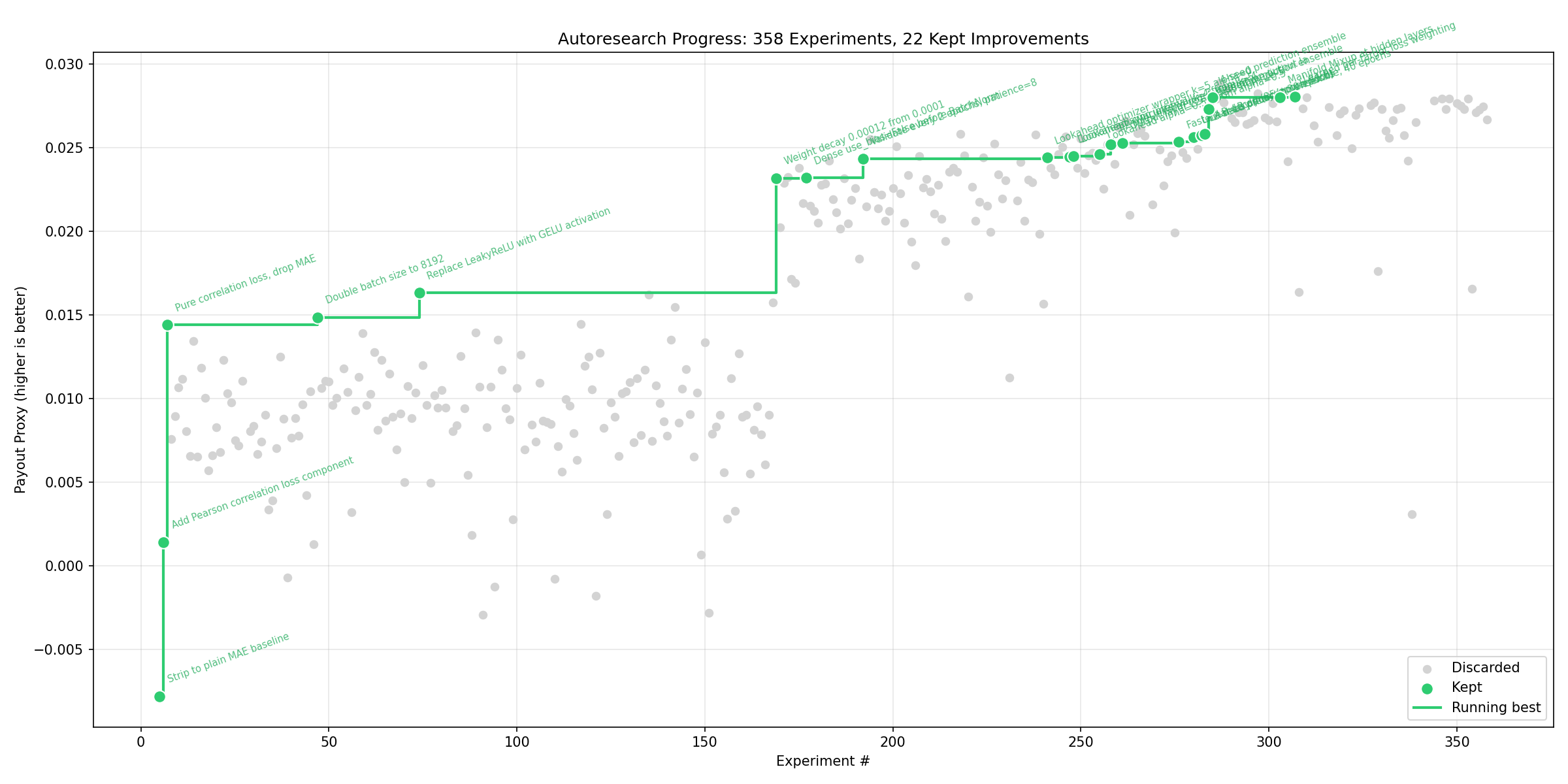
TL;DR: I adapted Karpathy’s autoresearch to optimize a neural network for the Numerai tournament. 358 autonomous experiments, 22 kept (6% hit rate), payout improved from -0.008 to 0.0280. Key adaptations: era-purged CV, multi-seed validation gates, synthesized learnings after each iteration, and a DO NOT RETRY table to prevent re-exploring exhausted search regions. Biggest surprise: every fancy tabular DL architecture (FT-Transformer, TabNet, GLU, MoE) lost to a plain 3-layer feedforward net with GELU.
In March 2026, Andrej Karpathy open-sourced autoresearch — a ~630-line Python tool that lets AI agents run autonomous ML experiments. The concept is elegant: give an LLM a train.py file, a fixed evaluation harness, and a research brief, then let it iterate. Each loop, the agent proposes a code change, trains the model, measures improvement, and commits or reverts. Overnight, you wake up to dozens of experiments and a Git history that reads like a lab notebook.
I adapted autoresearch to optimize a neural network for the Numerai tournament — a hedge fund competition where participants predict stock returns using anonymized financial features. 358 experiments later, payout improved from -0.008 to 0.0280, and I learned as much about what doesn’t work in tabular deep learning as what does.
This post covers what had to change when moving from language modeling to financial prediction, and what surprised me along the way.
Karpathy’s Original Design
The original autoresearch targets nanochat — a small character-level language model. The setup is minimal:
prepare.py: Fixed data loading and utilities (human-maintained)train.py: Editable model code (the agent modifies this)program.md: Research directions for the agent- Metric:
val_bpb(validation bits-per-byte) — a single scalar, lower is better - Budget: Fixed 5 minutes per experiment
- Loop: Prompt LLM → modify code → train → measure → commit or revert
The key insight is that the fixed time budget makes results comparable regardless of hardware, and the single metric makes improvement unambiguous. Shopify’s CEO reported a 19% improvement after 37 experiments overnight.
Why Numerai Is Harder
Numerai introduces several challenges that don’t exist in language modeling:
-
Composite metric: Payout isn’t just accuracy. It’s
0.75 * CORR20 + 2.25 * MMC, where MMC (Meta-Model Contribution) measures how much your predictions add to stake-weighted meta model. Being different matters 3x more than being accurate. -
Time-series structure: Financial data is grouped into eras — weekly in historical data, daily in the live tournament. Targets are 60-day forward returns, so adjacent eras have overlapping prediction windows. Naive train/val splits leak future information.
-
High noise floor: Stock returns are inherently noisy. The standard deviation of payout across cross-validation folds is ~0.005, meaning improvements smaller than ~1.3% of baseline are indistinguishable from random variance.
-
Anonymized features: You can’t reason about feature semantics — no “price”, “volume”, or “momentum”. Numerai v5.2 provides 2,748 features total, but we locked the agent to 235 features from the “serenity” and “wisdom” subsets (chosen for their high BMC Sharpe ratios) to keep experiment cycle times short. Future autoresearch runs will explore the full feature set.
-
Benchmark orthogonalization: BMC (Benchmark Model Contribution – a proxy for MMC) is computed by removing the signal that Numerai’s existing LightGBM ensemble already captures. Your neural net must find signal that gradient-boosted trees miss.
Dataset Configuration
All experiments used Numerai dataset v5.2 with the following configuration:
| Parameter | Value |
|---|---|
| Dataset version | v5.2 |
| Training set | “normaltrain” (2.7M rows, 574 eras) |
| Features | “serenity” (95) + “wisdom” (140) = 235 of 2,748 available |
| Targets | 20 target columns with 60-day forward returns (e.g. target_alpha_60, target_bravo_60) |
| Scoring target | target (primary Numerai evaluation target) |
| Era downsampling | Every 4th era (~143 training eras) for faster iteration |
| Validation | Last 50 eras held out |
| Cross-validation | 4-fold era-purged CV with 8-era embargo |
The benchmark ensemble (bm_ensemble) is the mean of all 8 LightGBM benchmark models provided in the v5.2 dataset: v52_lgbm_cyrusd20, v52_lgbm_teager2b20, v52_lgbm_ender20, v52_lgbm_jasper20, and their 60-day variants. This is broader than Numerai’s official V5_LGBM_CT_BLEND (a 50/50 blend of only Cyrus and Teager), since it also includes Ender and Jasper. BMC is computed by orthogonalizing our model’s predictions against this ensemble — any signal the LightGBMs already capture is subtracted out, and only the residual correlation with the target counts.
The feature subsets and era downsampling were locked in prepare.py as human decisions to keep experiment cycle times under 5 minutes per fold. The agent could modify everything in train.py (architecture, loss, optimizer, regularization) but could not change the data configuration.
The 10 Adaptations
1. Composite Evaluation Metric
Original: val_bpb — a single loss value from training.
Adapted: payout_proxy = 0.75 * mean_corr + 2.25 * mean_bmc
The evaluation function in prepare.py computes per-era Pearson correlation and per-era BMC (via orthogonalization against the benchmark ensemble), averages across eras, then combines them using the live payout formula. This means the agent optimizes for tournament performance, not just model accuracy.
def evaluate(predictions, val_df, target_columns):
    # Per-era correlation and BMC
    payout_proxy = 0.75 * mean_corr + 2.25 * mean_bmc
    return {"payout_proxy": payout_proxy, "mean_corr": mean_corr,
            "mean_bmc": mean_bmc, "sharpe_bmc": sharpe_bmc}
2. Era-Purged Cross-Validation
Original: Single train/validation split.
Adapted: 3-fold era-purged CV with 8-era embargo on each side.
Because targets are 60-day forward returns, adjacent eras have overlapping prediction windows. A standard k-fold split would leak information. Our CV assigns contiguous era blocks to folds and drops 8 eras on each side of the test block boundary. With weekly eras, that’s ~56 days of embargo — close to the 60-day target window. With ERA_DOWNSAMPLE=4 (every 4th era for faster iteration), the effective embargo is even wider.
# Era-purged CV: contiguous blocks with embargo
embargo_eras = 8  # eras on each side of test block
# ~56 days with weekly eras, prevents 60-day target leakage
This is slower (3x training per experiment vs. 1x) but prevents the most dangerous form of overfitting in financial ML. See the Numerai forum post on era-wise CV for background.
3. Multi-Seed Validation Gate
Original: Single training run determines keep/discard.
Adapted: Candidates must pass a 3-seed average validation before being kept.
Given the high noise floor, a single lucky seed can produce a spurious “improvement.” When the initial run beats the best, we re-train with seeds 17 and 73 (in addition to the original seed 42) and only keep the result if the 3-seed average exceeds the current best:
# Multi-seed validation in run.sh
for EXTRA_SEED in 17 73; do
    SEED_RESULT=$(... train_and_evaluate(data, seed=$EXTRA_SEED) ...)
    SEED_RESULTS="$SEED_RESULTS $SEED_PAYOUT"
done
AVG_PAYOUT=$(echo "$SEED_RESULTS" | awk '{s+=$1} END {printf "%.10f", s/NR}')
# Only KEEP if 3-seed average > best
This is critical — without it, the 6% hit rate would likely be much higher but filled with false positives.
4. Domain-Specific Research Brief (program.md)
Original: Generic ML research directions.
Adapted: 265-line document encoding Numerai domain knowledge.
The program.md file teaches the agent about BMC, the payout formula, feature set properties, hardware constraints (M3 Max with Metal backend — no CUDA), and time budgets per fold. The agent needs this context to make intelligent architecture choices. For example, knowing that BMC rewards orthogonality to tree ensembles steers the agent toward architectures that learn non-linear interactions that gradient boosting misses.
5. Knowledge Accumulation (learnings.md)
Original: No structured knowledge persistence between iterations.
Adapted: After every iteration, a second Claude call synthesizes results into a structured learnings file.
This is the most impactful adaptation. After each experiment, the run loop invokes Claude again with the diff, the result, and the current learnings, asking it to synthesize (not append) observations:
# Post-eval analysis in run.sh
claude -p "You are reviewing autoresearch iteration $i.
Status: $STATUS, payout_proxy: $PAYOUT...
Update learnings.md with structured, synthesized observations."
The resulting learnings.md is organized by category (architecture, loss, optimizer, regularization, etc.) and distinguishes “confidently bad” (tried 3x, always worse) from “ambiguous” (mixed results across seeds). By iteration 358, this file contains the distilled knowledge of every experiment — a compressed search history that prevents the agent from wasting iterations on exhausted directions.
6. Near-Miss Analysis
Original: No feedback on close failures.
Adapted: near_misses.py extracts the top 3 discarded experiments closest to beating the current best and feeds their diffs to the agent.
Near-misses are often more informative than clear failures. A change that achieved 99.5% of the best payout might be one small tweak away from an improvement. By showing the agent what almost worked, we give it a more productive starting point than a blank slate.
7. Phase-Based Search Strategy
Original: Uniform search strategy throughout.
Adapted: 8 phases that shift from exploration to exploitation to architectural innovation:
| Phase | Iterations | Strategy |
|---|---|---|
| 1 | 1-25 | Single focused changes, explore broadly |
| 2 | 26-50 | Combine 2-3 changes, mix near-misses |
| 3 | 51-75 | Fundamentally different approaches |
| 4 | 76-267 | Exploit best region, small perturbations |
| 5 | 268-300 | Evaluation robustness (multi-seed, 5-fold) |
| 6 | 301-350 | Tabular-specific architectures (FT-Transformer, TabNet) |
| 7 | 351-400 | Training paradigm shifts (SAM, Manifold Mixup) |
| 8 | 401+ | Ensemble diversity for BMC maximization |
Each phase is communicated to the agent as part of the prompt, steering its creativity toward the most productive frontier.
8. Plateau Detection
Original: No mechanism to detect stalled progress.
Adapted: After 15 consecutive discards, the agent receives an explicit hint to try fundamentally different approaches.
if [ "$CONSECUTIVE_DISCARDS" -ge 15 ]; then
    PLATEAU_HINT="IMPORTANT: $CONSECUTIVE_DISCARDS consecutive experiments
    have been discarded. Consider switching to a fundamentally different
    approach or combining near-misses."
fi
Without this, the agent tends to make increasingly marginal changes in the same neighborhood, burning iterations on noise-level variations.
9. DO NOT RETRY Table
Original: The agent tracks what it’s tried via Git history, which gets long and hard to parse.
Adapted: A structured table in program.md listing 20+ exhaustively searched categories with trial counts.
| Category | Status | Details |
|---|---|---|
| Feedforward width/depth | EXHAUSTED (15+) | [512,256,128] optimal |
| Activations | EXHAUSTED (10+) | GELU optimal. Swish -35%, Mish -67% |
| Dropout | EXHAUSTED (8) | 0.2 uniform optimal |
| ...20 more categories... |
After learnings.md, this is the second most effective mechanism for preventing wasted iterations. Without it, the agent would repeatedly try dropout 0.15 or Swish activation — changes that have been conclusively ruled out.
10. Production Integration
Original: Results stay in the research loop.
Adapted: The winning configuration is promoted to a production module (dp32_autoresearch_nn/) that runs in the daily submission pipeline.
This closes the loop from research to deployment. The best autoresearch iteration’s hyperparameters and architecture are copied to a standalone module with --train, --predict, and --submit CLI flags, integrated into the daily submission run.
Results: 358 Experiments in Numbers
| Metric | Value |
|---|---|
| Total experiments | 358 |
| Kept (improvements) | 22 (6.1%) |
| Discarded | 308 (86.0%) |
| Errors | 28 (7.8%) |
| Starting payout | -0.008 |
| Final payout | 0.0280 |
| Categories searched | 20+ |
| Hyperparameter axes exhausted | All major ones |
The 6% hit rate is deceptive — it includes multi-seed validation, which filters out roughly half of initially-promising candidates. Without multi-seed gating, the apparent hit rate would be ~12%, but many of those “improvements” would be noise.
Key Improvements Over Baseline
The biggest gains came from a few decisive changes:
| Change | Improvement | Iteration |
|---|---|---|
| Pure Pearson correlation loss (drop MAE) | +inf (baseline was negative) | Early |
| GELU activation | +13% | Early |
| Weight decay 0.00012 | +42% | Mid |
| Batch size 8192 | +3% | Early |
| 4-seed prediction ensemble | +9% | 285 |
| Lookahead optimizer (k=3, alpha=0.55) | +1.2% | Mid |
| Output L2 regularization 2.5e-5 | +2.4% | Mid |
The Final Architecture
[512, 256, 128] GELU + HeUniform initialization
Dense(use_bias=False) -> BatchNorm -> GELU -> Dropout(0.2)
Manifold Mixup (alpha=0.4, random hidden layer)
Learned per-target loss weights (softmax logits, temp=2.0)
AdamW(lr=0.001, wd=0.00012, clipnorm=1.0) + Lookahead(k=3, alpha=0.55)
PolynomialDecay (30 epochs, end_lr=0.1x)
4-seed prediction ensemble (avg predictions from seeds 42, 142, 242, 342)
40 epochs, batch 8192, patience 8
Remarkably simple. After 358 experiments across transformers, gating mechanisms, mixture-of-experts, and exotic regularizers — a plain feedforward network with batch normalization won.
Surprising Findings
Tabular Deep Learning Architectures All Failed
This was the biggest surprise. FT-Transformer (the #1 tabular DL method in academic benchmarks) scored -21%. TabNet, GLU layers, DCN-v2, Mixture of Experts — all worse than the simple feedforward baseline. Every structured attention mechanism, every gating variant, every architecture designed specifically for tabular data underperformed three Dense layers with GELU.
Hypothesis: With only 235 features (from the locked subset) and ~143K training rows (after era downsampling), the data can’t support the parameter overhead of attention mechanisms. Tabular DL benchmarks typically use much larger datasets. This may change when future runs use the full 2,748-feature set. Also, Numerai’s pre-normalized [0,1] features may already be in a representation where learned feature embeddings add no value.
Ensemble Diversity Hurts
The 4-seed prediction ensemble (training 4 identical models with different seeds, averaging predictions) gave a +9% improvement — the single biggest gain after the initial configuration. But every attempt to introduce diversity between the seeds made things worse:
- Per-seed learning rate diversity: noise to -5%
- Per-seed schedule diversity (linear/cosine/sqrt): -4%
- Per-seed architecture diversity: -1% to -2%
- Per-seed dropout diversity: -7%
- NCL diversity penalty: -37%
- Rank-based aggregation: -2%
The paradox: Variance reduction through averaging identical models beats all diversity strategies. The optimal ensemble is four copies of the same thing.
You Can’t Exploit the Benchmark
Since BMC measures orthogonal contribution relative to Numerai’s LightGBM ensemble, an obvious strategy is to explicitly learn the residual — predict what the benchmark gets wrong. Every attempt failed:
- Residual learning (predict target minus benchmark): -16% to -54%
- BMC as a loss component: -33%
- Stop-gradient on benchmark predictions: -48%
- BMC-aware early stopping: -2%
The benchmark ensemble is either too noisy to learn from or already captures the learnable signal along that direction. The neural network finds orthogonal signal incidentally, not by trying.
Noise Dominates Everything
The no-change retest standard deviation is 0.0048. With the best payout at 0.0280, that means improvements below 1.3% of baseline (~0.00036 absolute) are literally indistinguishable from re-running the same code with a different random seed. Many experiments that showed “102-104% of best” with high fold standard deviation were not reproducible.
This is the fundamental challenge of financial ML — and why the multi-seed validation gate and DO NOT RETRY table are not just nice-to-haves but essential infrastructure.
What Worked About the Approach
Knowledge accumulation is the killer feature. The learnings.md synthesis after each iteration means the agent gets smarter over time. By iteration 300, the agent has internalized which regions of the search space are exhausted and can focus on genuinely novel directions. Without this, I estimate at least 30-40% of iterations would be wasted on re-exploring dead ends.
The bash loop is surprisingly robust. The entire orchestration is a 345-line bash script (run.sh) that calls claude -p with constructed prompts. No framework, no agent SDK, no LangChain. Just bash, jq, bc, and Claude. It handles timeouts, NaN detection, git operations, multi-seed validation, and plateau detection. I ran it overnight for multiple sessions without intervention.
The agent is remarkably good at implementing ML ideas. Claude consistently produced working TensorFlow code for complex architectures (FT-Transformer, Manifold Mixup with custom train_step, learned loss weights). The 7.8% error rate is low considering the diversity of changes attempted.
What I’d Do Differently
Start with multi-seed evaluation from iteration 1. The early iterations (1-267) used single-seed evaluation, and I suspect several “improvements” during that phase were noise. The multi-seed gate should have been the default from the start.
Use a larger validation set. Era downsampling to ~143 eras keeps training fast but makes the signal-to-noise ratio punishing. With more validation data, smaller improvements would be detectable.
Try fundamentally different model families earlier. Phases 1-4 spent 267 iterations tuning a feedforward network. The later phases (tabular architectures, training paradigms) produced the most interesting findings but had fewer iterations to explore them.
Track wall-clock cost. Each experiment takes 10-20 minutes (3-fold CV x 4 prediction seeds x ~3 min/fold). 358 experiments is roughly 60-120 hours of compute on a MacBook. Tracking cost per improvement would help decide when to stop.
Conclusion
Adapting autoresearch to Numerai required confronting the hardest parts of financial ML: noisy signals, time-series leakage, composite metrics, and the fundamental challenge of finding signal orthogonal to an existing ensemble. The 10 adaptations — from era-purged CV to the DO NOT RETRY table — are transferable to any domain where the evaluation is noisy, the metric is complex, or the search space is large.
The most counterintuitive finding is that after 358 experiments spanning 20+ categories, the winning architecture is three Dense layers with GELU. No attention, no gating, no mixture of experts. Sometimes the simplest architecture is the right one — you just need 358 experiments to be confident of that.
The winning model is submitted daily to the Numerai tournament as david_plutus_32 — you can track its live performance there.